using CSV
using DataFrames
y = DataFrame(CSV.File("CCLE-ActArea.csv")).:"PD-0325901" #select(DataFrame(CSV.File("CCLE-ActArea.csv")), :"PD-0325901")
X = DataFrame(CSV.File("CCLE-expr.csv"))Solving the data leakage problem with learning networks
Julia
MLJ
Genomics
Machine learning
Tom Michoel 
The data leakage problem
Nowadays every student who has taken a basic course in machine learning is aware of the problem of data leakage and the need for proper separation between training, validation, and test data sets. Nonetheless, survey after survey shows that data leakage is pervasive in ML-based science. How can this discrepancy be explained?
Part of the problem, I believe, is that most ML courses make use of standard, ready-made datasets for putting theory into practice (anyone out there who hasn’t used the MNIST database?). In real life though, and certainly in biology, there is a long series of preprocessing steps to go from raw data to the nice \(X\) and \(y\) array inputs one uses in ML (check out some of the workflows on the Galaxy project to get an idea how complex data preprocessing can be).
These preprocessing workflows are often not run with later ML applications in mind, and often not even by the same person who will do the ML modelling. This leads to plenty of opportunity for data leakage. The pitfalls of leaky preprocessing have been well described (make sure also to memorize the other pitfalls described in the same article!).
What can be done to avoid leaky preprocessing? Learning networks, are the answer! Learning networks, not to be confused with deep learning or neural networks, are, in the words of its authors, simple transformations of your existing workflows which can be “exported” to define new, re-usable composite model types (models which typically have other models as hyperparameters) (see also this blog post and the technical paper).
Let’s break this down in two parts: how model composition can eliminate data leakage and what additional flexibility is offered by learning networks.
A linear pipeline: variable gene selection
We will use gene expression and drug sensitivity data from the first cancer cell line encyclopedia paper. A copy of (the relevant part of) the data is available on JuliaHub and consists of expression data for 18,926 genes and sensitivity data for 24 drugs in 474 cancer cell lines. We load data for one specific drug as our response variable \(y\) and expression data for all genes as our predictor matrix \(X\):
Since so many genes are profiled in a relatively small number of samples, many will not show much variation:
using Plots
using Statistics
sd = map(x -> std(x), eachcol(X))
histogram(sd; xlabel="Standard deviation", label="")
Therefore it is common to keep only variable genes (for instance, using a cutoff on the standard deviation) for downstream analysis. However, if we simply remove genes with low standard deviation at this point, we enter the leaky preprocessing terrain, because information from all samples has been used to compute the standard deviations.
The common solution is to first split data in training, validation, and test datasets, and then do the filtering on the training data alone. This is messy and prone to errors because one has to keep track manually of the different datasets.
A much better solution is to create a linear pipeline composed of two models: a feature selection model and a regression model.
The feature selection model
We want to keep the standard deviation threshold as a parameter of the feature selection model, which does not seem possible with MLJ’s built-in FeatureSelector. Hence we define a new unsupervised model:
using MLJ
import MLJModelInterface
MLJModelInterface.@mlj_model mutable struct FeatureSelectorStd <: Unsupervised
    threshold::Float64 = 1.0::(_ > 0)
end

function MLJ.fit(fs::FeatureSelectorStd, verbosity, X)
    # Find the standard deviation of each feature
    stds = map(x -> std(x), eachcol(X))
    selected_features = findall(stds .> fs.threshold)
    cache = nothing
    report = nothing
    return selected_features, cache, nothing
end

function MLJ.transform(::FeatureSelectorStd, fitresult, X)
    # Return the selected features
    return selectcols(X,fitresult)
end
A trivial but nonetheless important point is that the fit function identifies the features with standard deviation greater than the threshold from its argument \(X\), while the transform function applies the feature selection to a possibly different \(X'\), irrespective of the standard deviation values in that \(X'\). To illustrate this, let’s fit a feature selector on all but the first cell line, and use it to transform the left-out one. First we create a machine that binds our feature selector (with default standard deviation threshold of 1) to the selected samples, then we fit the machine to the data (that is, compute the standard deviation of each feature and find the ones exceeding the threshold), and finally transform (i.e., select the relevant features from) the held-out sample:
mfs = machine(FeatureSelectorStd(),selectrows(X,2:nrow(X)));
fit!(mfs)
MLJ.transform(mfs,selectrows(X,1))
Creating a feature selection model with a different standard deviation threshold is as simple as
FeatureSelectorStd(threshold=2.0)FeatureSelectorStd(
threshold = 2.0)The regression model
To predict drug sensitivity from gene expression data, we will use random forest regression. The model is imported as follows:
using MLJDecisionTreeInterface
RandomForestRegressor = @load RandomForestRegressor pkg="DecisionTree";
[ Info: For silent loading, specify `verbosity=0`. import MLJDecisionTreeInterface ✔
The pipeline model
A linear pipeline model that first performs feature selection and then random forest regression with default parameter values is easily constructed:
fs_rf_model = FeatureSelectorStd() |> RandomForestRegressor()DeterministicPipeline(
feature_selector_std = FeatureSelectorStd(
threshold = 1.0),
random_forest_regressor = RandomForestRegressor(
max_depth = -1,
min_samples_leaf = 1,
min_samples_split = 2,
min_purity_increase = 0.0,
n_subfeatures = -1,
n_trees = 100,
sampling_fraction = 0.7,
feature_importance = :impurity,
rng = Random.TaskLocalRNG()),
cache = true)A pipeline model can be fitted and evaluated like any other MLJ model, see the common MLJ workflows.
fs_rf_mach = machine(fs_rf_model,X,y)
train, test = partition(1:nrow(X), 0.8, shuffle=true)
fit!(fs_rf_mach, rows=train)
yhat = predict(fs_rf_mach, X[test,:])scatter(y[test], yhat; label="", xlabel="True response", ylabel="Predicted response")
By incorporating data preprocessing steps in the ML model, we avoid having to remember to split the data before any preprocessing, giving a lot more flexibility in the analysis and avoiding data leakage. The real beauty though is perhaps that the preprocessing parameters (here, standard deviation threshold) become learnable hyperparameters of the combined model! In other words, instead of setting preprocessing parameters to some arbitrary value without clear justification, as is common in bioinformatics pipelines, we can now tune their value to the learning goal (finding the best model to predict drug sensitivity from gene expression).
As an example, we tune the standard deviation threshold using grid search and 5-fold cross-validation on the training data, while keeping the default parameters for the random forest regressor (following this tutorial):
r = range(fs_rf_model, :(feature_selector_std.threshold), lower=0.5, upper=3.0)
tuned_fs_rf_model = TunedModel(
    model=fs_rf_model,
    resampling=CV(nfolds=5),
    tuning=Grid(resolution=20),
    range=r,
    measure=rms
)
tuned_fs_rf_mach = machine(tuned_fs_rf_model, X, y)
fit!(tuned_fs_rf_mach, rows=train)
fitted_params(tuned_fs_rf_mach)[:best_model]
We find that the best standard deviation threshold is 1.5526315789473684. The average RMS at each threshold can be plotted:
plot(tuned_fs_rf_mach)
Linear pipelines can obviously contain multiple preprocessing steps. For instance, here is a pipeline that first performs variable gene selection followed by standardizing each gene to mean 0 and standard deviation one, followed by a regression model1:
using MLJTransforms
Standardizer = @load Standardizer pkg=MLJTransforms
FeatureSelectorStd() |> Standardizer() |> RandomForestRegressor()
[ Info: For silent loading, specify `verbosity=0`. import MLJTransforms ✔
DeterministicPipeline(
  feature_selector_std = FeatureSelectorStd(
        threshold = 1.0),
  standardizer = Standardizer(
        features = Symbol[],
        ignore = false,
        ordered_factor = false,
        count = false),
  random_forest_regressor = RandomForestRegressor(
        max_depth = -1,
        min_samples_leaf = 1,
        min_samples_split = 2,
        min_purity_increase = 0.0,
        n_subfeatures = -1,
        n_trees = 100,
        sampling_fraction = 0.7,
        feature_importance = :impurity,
        rng = Random.TaskLocalRNG()),
  cache = true)
A learning network: supervised gene selection
In the previous example we selected genes based on their variability. But since we’re ultimately interested in building a predictive model for the response variable (drug sensitivity), would it not make more sense to select genes based on their correlation with the response? In lasso regression, features are guaranteed to be absent in the optimal model if their correlation with the response is sufficiently small (so-called safe feature elimination). In genomics, when constructing polygenic scores, it is common to select features (in this case, SNPs) based on their effect size (that is, correlation with the outcome) in the corresponding GWAS. According to Barnett et al (2022), using the entire dataset for GWAS and this kind of feature selection is the most common form of data leakage in this area.
A feature selection step that depends on the target variable \(y\) cannot be put in a linear pipeline, because at most one the pipeline components may be a supervised model2. What we need instead is a workflow like this:
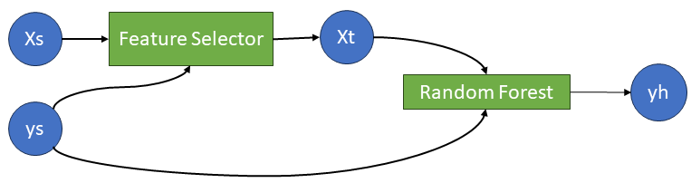
Learning networks are exactly what is needed to implement such a model.
The supervised feature selection model
First we construct our feature selector:
MLJModelInterface.@mlj_model mutable struct FeatureSelectorCor <: Unsupervised
    threshold::Float64 = 0.1::(_ > 0)
end

function MLJ.fit(fs::FeatureSelectorCor, verbosity, X, y)
    # Find the correlation of each feature with y
    cors = map(x -> abs(cor(x,y)), eachcol(X))
    selected_features = findall(cors .> fs.threshold)
    cache = nothing
    report = nothing
    return selected_features, cache, nothing
end

function MLJ.predict(::FeatureSelectorCor, fitresult, X, y)
    # Return the selected features
    return selectcols(X,fitresult)
end

function MLJ.transform(::FeatureSelectorCor, fitresult, X)
    # Return the selected features
    return selectcols(X,fitresult)
end
The learning network
Now we construct the learning network, pretty much following the documentation.
First the data source nodes:
Xs = source(X);
ys = source(y);
Now the feature selector machine and the transformed feature data node:
mach_fs = machine(FeatureSelectorCor(threshold=0.2),Xs, ys);
Xt = MLJ.transform(mach_fs,Xs);
Then the random forest regression machine and the predicted response node:
mach_rf = machine(RandomForestRegressor(), Xt, ys)
yh = predict(mach_rf,Xt);
To fit the learning network on the training samples, we call fit! on the output node, which triggers training of all the machines on which it depends:
fit!(yh, rows=train);[ Info: Training machine(FeatureSelectorCor(threshold = 0.2), …). [ Info: Training machine(RandomForestRegressor(max_depth = -1, …), …).
The fitted model can be compared to the true values on the test samples using the syntax yh(rows=test); the RMSE in this case is 1.139342678014389
scatter(y[test],yh(rows=test), label="", xlabel="True response", ylabel="Predicted response")
Exporting the learning network as a new model type
A learning network must be exported as a new model type to allow hyperparameter tuning. This has the additional benefit that the feature selector and regression model can easily be swapped for alternative models. We follow the documentation and first define a new composite model type with the same supertype as a random forest regressor:
supertype(typeof(RandomForestRegressor()))DeterministicOur new composite model consists of a feature selector and a regressor:
mutable struct CompositeFS <: DeterministicNetworkComposite
    featureselector
    regressor
end
No we need to make our learning network generic and wrap it in a prefit method:
import MLJBase
function MLJBase.prefit(composite::CompositeFS, verbosity, X, y)

    # the data source nodes
    Xs = source(X)
    ys = source(y)

    # the supervised feature selector
    mach_fs = machine(:featureselector, Xs, ys);
    Xt = MLJ.transform(mach_fs,Xs)

    # the regressor on the preprocessed data
    mach_regr = machine(:regressor, Xt, ys)
    yhat = predict(mach_regr, Xt)

    verbosity > 0 && @info "I'm a learning network"

    # return "learning network interface":
    return (; predict=yhat)
end
An instance of the new model type is created and fitted using the standard interface
composite_fs_model = CompositeFS(FeatureSelectorCor(), RandomForestRegressor())
mach_composite_fs = machine(composite_fs_model, X, y)
fit!(mach_composite_fs, rows=train)
yhat = predict(mach_composite_fs, X[test,:])
scatter(y[test], yhat; label="", xlabel="True response", ylabel="Predicted response")
[ Info: Training machine(CompositeFS(featureselector = FeatureSelectorCor(threshold = 0.1), …), …). [ Info: I'm a learning network [ Info: Training machine(:featureselector, …). [ Info: Training machine(:regressor, …).

Tuning the preprocessing hyperparameter
Using the new model type, we can tune the correlation threshold, keeping the default random forest hyperparameters:
r = range(composite_fs_model, :(featureselector.threshold), lower=0.05, upper=0.35)
tuned_composite_fs_model = TunedModel(
    model=composite_fs_model,
    resampling=CV(nfolds=5),
    tuning=Grid(resolution=20),
    range=r,
    measure=rms
)
tuned_composite_fs_mach = machine(tuned_composite_fs_model, X, y)
fit!(tuned_composite_fs_mach, rows=train)fitted_params(tuned_composite_fs_mach)[:best_model]CompositeFS(
featureselector = FeatureSelectorCor(
threshold = 0.2868421052631579),
regressor = RandomForestRegressor(
max_depth = -1,
min_samples_leaf = 1,
min_samples_split = 2,
min_purity_increase = 0.0,
n_subfeatures = -1,
n_trees = 100,
sampling_fraction = 0.7,
feature_importance = :impurity,
rng = Random.TaskLocalRNG()))plot(tuned_composite_fs_mach)
Footnotes
This is of course a hypothetical example, a random forest regressor does not need any standardization or other type of scaling, because it only cares about the order of values of a feature, not their absolute value.↩︎
The pipeline documentation states that “Some transformers that have type Unsupervised (so that the output of transform is propagated in pipelines) may require a target variable for training […]. Provided they appear before any Supervised component in the pipelines, such models are supported.” In theory this should apply to a
FeatureSelectorCor, but including one in a linear pipeline gives an error during fitting. Maybe I’ve not understood how to do this properly?↩︎