Luria-Delbrück fluctuation experiment
A Luria-Delbrück fluctuation experiment consists of growing many independent clones from single cells (or organisms), all under the same conditions but each starting from a (possibly different) initial state. The key quantity of interest is the distribution of some summary statistic — such as the number of mutant cells — across clones.
The fluctuation_experiment function provides a convenient shortcut for this workflow. It takes a ConstantRateBranchingProblem, a distribution from which initial states are sampled independently for each clone, and the number of clones to simulate. Internally it uses SciML's EnsembleProblem interface and automatically applies reduce_tree to each clone's branching tree, returning an EnsembleSolution of ReducedBranchingProcessSolution objects.
Setting up the problem
We model the classical Luria-Delbrück experiment as a birth-death process in which a wild-type cell (W) can acquire a mutation and become a mutant cell (M), with no back-mutations:
using Catalyst
rn = @reaction_network begin
    μ, W --> M
end
u0 = [:W => 1, :M => 0]
p  = [:μ => 0.1]
tspan = (0.0, 5.0)
We set up the corresponding JumpProblem and wrap it in a ConstantRateBranchingProblem:
using StochasticDiffEq, JumpProcesses
jprob  = JumpProblem(rn, u0, tspan, p)

using BranchingProcesses
λ      = 1.0   # branching (cell division) rate
nchild = 2     # each cell divides into two daughter cells
bjprob = ConstantRateBranchingProblem(jprob, λ, nchild);
Running a fluctuation experiment
In this model every clone starts from the same initial condition (one wild-type cell, zero mutants). We encode this as a product_distribution of two Dirac distributions:
using Distributions
u0_dist = product_distribution([Dirac(1), Dirac(0)])
We then call fluctuation_experiment to simulate 100 independent clones. Each clone starts from a fresh sample drawn from u0_dist, and the branching tree is immediately reduced (summed over all live cells) via solve_and_reduce:
results = fluctuation_experiment(bjprob, u0_dist, 100;
                                 alg=SSAStepper(),
                                 ensemble_alg=EnsembleThreads(),
                                 reduce_kwargs=(; output_dt=0.1));
results is an EnsembleSolution whose elements are ReducedBranchingProcessSolution objects. We can inspect a single clone's reduced time series:
using Plots
plot(results.u[1])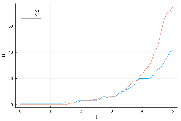
Visualising the distribution across clones
The main interest in a fluctuation experiment is the distribution of a quantity across clones at the end of the experiment. We extract the number of mutant cells (M, index 2) at the final time for each clone:
mutant_counts = [sol.u[end][2] for sol in results.u]
histogram(mutant_counts; #bins=0:maximum(mutant_counts)+1,
          xlabel="Mutant cell count", ylabel="Number of clones",
          label="", title="Luria-Delbrück distribution")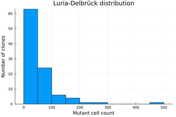
The characteristic feature of the Luria-Delbrück distribution is its heavy tail: most clones have few or no mutants, while a small number of "jackpot" clones carry many mutants due to early mutations.
A custom reduction and rescaling function
By default fluctuation_experiment uses sum to aggregate cell values at each time point, but any callable is accepted. For instance, to track the maximum value across independent realizations of a branching Brownian motion with initial states sampled ranomdly from a standard normal:
f(u,p,t) = 0.0
g(u,p,t) = 1.0

bm = SDEProblem(f, g, 0.0, (0.0, 5.0))
bbm = ConstantRateBranchingProblem(bm, λ, 2)

u0_dist = Normal(0.0, 1.0)
results_max = fluctuation_experiment(bbm, u0_dist, 20;
alg=EM(), solver_kwargs=(; dt=0.01),
reduction=maximum,
ensemble_alg=EnsembleThreads());
plt2 = plot(; xlabel="t", ylabel="max over cells", legend=false)
for sol in results_max.u
plot!(plt2, sol)
end
plt2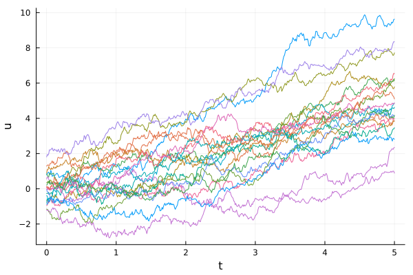
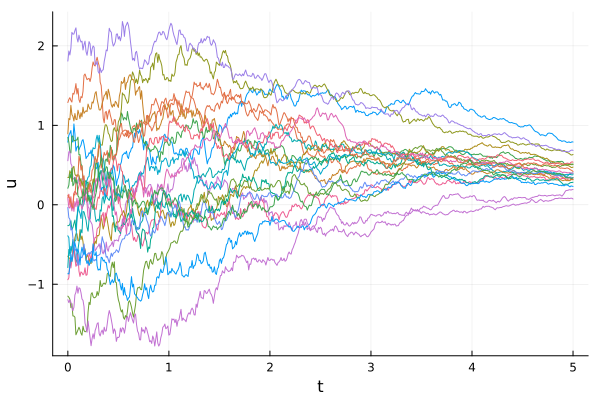
The reduction function is by definition the same at all time points. Time-dependency can be introduced by scaling each clone's reduced solution by a time-dependent factor. For instance, to rescale the maximum value in the previous experiment by the square root of the expected number of particles $e^{\lambda t}$:
rescale_fun = t -> exp(-0.5*λ*t)
results_max_scaled = fluctuation_experiment(bbm, u0_dist, 20;
                                     alg=EM(), solver_kwargs=(; dt=0.01),
                                     reduction=maximum,
                                     rescale=rescale_fun,
                                     ensemble_alg=EnsembleThreads());
plt3 = plot(; xlabel="t", ylabel="rescaled max over cells", legend=false)
for sol in results_max_scaled.u
    plot!(plt3, sol)
end
plt3